Understanding relationships between species and their habitats is important to the successful conservation and management of wildlife populations. Inferring how current and future habitat conditions affect wildlife population dynamics is critical when making adaptive decisions about land and resource use in the face of ecological change. In many cases, quantifying relationships between the quality and distribution of habitat and the abundance and distribution of wildlife populations can be valuable for evaluating land conservation and harvest management options (C. J. Johnson & Rea, 2024; Mateen et al., 2025; Schrempp et al., 2019; Street et al., 2015). For example, quantifiable wildlife-habitat relationships can be particularly useful when making strategic land management decisions over large landscapes using decision-making tools such as the Resist-Accept-Direct framework developed for response to ecological transformation (Lynch et al., 2021; Schuurman et al., 2022; Thompson et al., 2020).
Quantifying wildlife-habitat relationships often involves relating measures of population abundance or occurrence to habitat conditions within an appropriate modeling framework. To make that link, animal locations must be spatially related to environmental features important to a species’ life history traits at those locations. Animal locations can be collected using a variety of methods, including animal tracking devices (e.g., VHF or GPS tracking collars), handheld GPS units, and spatially referenced photographs. Environmental data begin as spatially referenced information formatted as points, lines, polygons, or rasters in a geographical information system and are subsequently used to extract or calculate the environmental features to be included in models used to estimate wildlife-habitat relationships.
When relating animal locations to environmental data, analysts commonly ignore measurement errors associated with those locations, or assume errors are absent or negligible compared to other sources of variation in the data. For many GPS-based field methods used to remotely collect animal locations (e.g., GPS tracking collars), researchers often assume measurement errors are negligible during analysis due to the relatively high accuracy and precision of GPS technology. However, that assumption may not be appropriate for other field methods that require observers to manually collect animal locations from fast-moving, non-stationary platforms, such as aircraft during aerial surveys, even when GPS devices are used to collect those locations. Therefore, determining and accounting for measurement bias and imprecision of animal locations is important when designing research studies or long-term monitoring programs to quantify and evaluate wildlife-habitat relationships.
Aerial surveying is a common field method used to study and monitor wildlife populations over large, inaccessible landscapes. For such surveys, observers commonly use handheld GPS devices to collect locations of individual animals or animal groups from a moving aircraft high above ground level (AGL). Location measurement error may increase under such circumstances due to differences in aircraft types, weather factors such as high winds, GPS device limitations, inaccurate communication between personnel in the aircraft, or pilot and observer position in the aircraft (Marques et al., 2006).
In this case study, our goal was to investigate the potential for measurement errors when collecting animal locations during aerial surveys to monitor moose (Alces alces) population abundance and spatial distribution at Yukon Delta National Wildlife Refuge (YKD) in western Alaska. Our objective was to estimate and compare measurement bias and precision of animal locations collected with handheld GPS devices during aerial surveys at YKD by simulating survey conditions from fixed-wing aircraft and helicopters using a target with a known location. For our fixed-wing survey, we expected locations to be positively biased in the direction of travel, due to linear aircraft movement at high speeds, and minimally biased in the left-right directions. We also hypothesized that greater airspeeds during fixed-wing trials could increase positive bias in the front-back direction. For helicopter trials, we did not expect bias in any direction due to minimal expected lateral movement of the aircraft while hovering to collect locations.
STUDY AREA
The study area was located at Hangar Lake near the village of Bethel in western Alaska. The location was chosen because of its convenience and proximity to Bethel and because of its familiarity to the two pilots involved in the study. Hangar Lake is located approximately 1.6 km east of Bethel and has a gravel road accessing it. A chain link fence gate located along Hangar Lake was chosen as the known landmark for the study because it was clearly visible from the air, precluding location error due to physical obstructions, and approximated the size of a moose. The area surrounding the gate was bordered by Hangar Lake to the east and by spruce (Picea spp.) and willow (Salix spp.) bog in all other directions. Little or no vegetation, snow, or ice were present on the lake within 9–15 meters of the gate during the study, thus ensuring clear visibility of the landmark from the AGL at which YKD aerial surveys are conducted.
METHODS
Our general approach was to conduct simulated aerial surveys during which locations were collected for a fixed landmark with known location and then compared with that known location to quantify measurement bias and precision. We based our simulated surveys on field methods common to aerial wildlife population monitoring in Alaska that entail a non-pilot observer using a handheld GPS unit to collect animal locations observed during a survey (Kellie & DeLong, 2006). We conducted simulated surveys using a fixed-wing airplane on 28 April 2022 and a helicopter on 29 April 2022 to allow comparison of measurement errors between survey platforms.
Field protocol
We used a Garmin GPSMAP 276Cx as the handheld GPS unit to determine the true location for the fixed landmark and for collecting locations during simulated surveys because that make and model was commonly used for aerial surveys at YKD. All locations were collected in the WGS84 coordinate system and reprojected to the USA Contiguous Albers Equal Area Conic for analysis. The true location of the fence gate at Hangar Lake used as our known landmark was determined by averaging 30 GPS waypoints collected on the ground at the center of the gate prior to fixed-wing surveys on 28 April 2022.
To simulate fixed-wing surveys, a 2-person survey team consisting of a pilot and a backseat observer used a Piper Supercub to fly over and collect 30 waypoints for the landmark. The pilot attempted to maintain an approximate AGL of 120 m and an airspeed of 125 kph while approaching the landmark from various different directions during each flyover. The survey team standardized their procedures in collecting waypoints by having the pilot calling out a countdown from 5 to 1 followed by a “mark” command when the pilot believed the aircraft was directly over the landmark, at which point the observer recorded a waypoint on the handheld GPS. After recording each location, the pilot would then fly approximately 1.5 km away from the landmark to approach from a new direction chosen by the pilot to collect the next location until a sample of 30 waypoints was collected. Track points were also collected by the GPS unit to record flight paths for simulated surveys that were then used to determine the direction of travel and aircraft speed at the time of collection for each waypoint.
We simulated helicopter surveys using a Robinson R44 helicopter with a different pilot than the airplane, and with the same observer and fixed landmark at Hangar Lake. The waypoint collection procedure used for these surveys had the aircraft approach from various different directions chosen by the pilot and hover at approximately 98 m AGL until the pilot believed the aircraft was directly over the landmark, at which point the pilot commanded “mark” and the observer recorded a waypoint on the handheld GPS. After each waypoint was collected, the pilot would fly >100 m away from the landmark to approach from a new direction to collect the next location until a sample of 30 waypoints was collected.
Regression analysis
We used simple linear regression and Bayesian estimation methods to evaluate the accuracy and precision of waypoints collected during simulated surveys relative to the known location of the fixed landmark. For the fixed-wing data, we first calculated measurement error in meters between each sample GPS waypoint and the known location in two directions, along and perpendicular to the direction of travel determined from GPS track points. We then used each sample of errors as a response variable in fitting 2 regression models, an intercept-only model to estimate waypoint bias and precision and a single-covariate model adding a regression term for aircraft speed (airspeed) in kph calculated from recorded track points. The covariate model was based on the hypothesis that bias increased with airspeeds observed during our simulated surveys.
For the helicopter data, we also calculated errors between the 30 GPS waypoints and the known location in both north-south and east-west azimuths, both centered on the known location. We chose these azimuths mostly out of convenience, but also because our directions of approach to the target and hovering maneuvers used to obtain waypoints did not indicate a need for any specific azimuths. As in the fixed-wing analysis, we used the sample of errors in each direction as a response variable, but only fit an intercept-only model because airspeed was predetermined to not likely be a factor influencing measurement error due to hovering maneuvers used to obtain waypoints essentially having no directional airspeed.
We fit regression models to 2 data sets for each survey platform, 1 including all waypoint locations and 1 with the most extreme outlier waypoint removed, to better understand the potential influence of outliers. We identified the outlier for each platform as the waypoint with the largest margin of error in either measurement direction. Given our relatively limited sample sizes, our reanalysis was designed to provide a measure of estimator sensitivity to the most extreme value observed for each platform.
Data formatting and analysis were conducted using R version 4.2.3 (R Core Team, 2023). Bayesian regression models were fit using JAGS (Plummer, 2014) via the jagsUI package (Kellner, 2024) in R. We fit all models using vague priors with $\alpha\sim Normal(0,\ 10,000)\ $(intercept), $\beta\sim Normal(0,\ 10,000)\ $(slope coefficient), and $\sigma\sim Uniform(0,\ 100)\ $(standard deviation). Point estimates and quantile-based 95% credible intervals for model parameters and derived values were calculated from their respective posterior distributions approximated from 3 chains of 100,000 MCMC samples after thinning by 100 and discarding 50,000 burn-in samples.
Misclassification analysis
To better understand potential impacts of measurement error for each survey platform in an applied analysis setting, we estimated the probability of misclassifying animal locations (θ) when georeferencing locations to grid-style spatial data sets such as relating animal locations to rasterized landcover data. For simplicity, we used the normally distributed error distribution estimated from the intercept-only model for each platform that we fitted to data sets with outliers removed. To estimate θ, we first assumed 3 different spatial resolutions of 30-m × 30-m, 90-m × 90-m, and 250-m × 250-m for the grid, and we assumed target animals were located at the centers of grid cells to emulate common analytical assumptions made for animal location and rasterized habitat data. We then derived a platform-specific posterior distribution of θ in each direction as the proportion of the error distribution, defined by values of and for each MCMC sample, that extended above 15 m or below -15 m for a 30-m resolution, above 45 m or below -45 m for a 90-m resolution, and above 125 m or below -125 m for a 250-m resolution.
RESULTS
Summary statistics
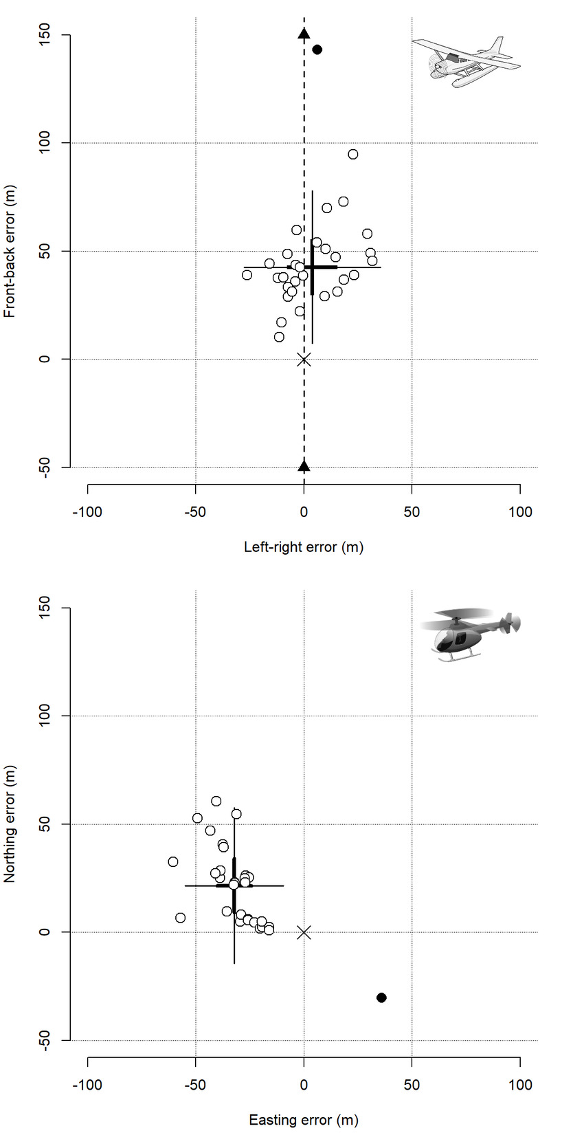
The sample mean x-coordinate (Easting) for the fixed landmark in UTM was 418,190.6 (SD = 0.61 m) and the sample mean y-coordinate (Northing) was 1,226,477.0 (SD = 0.46 m). The sample means of errors measured in the left-right (i.e., x axis), front-back (i.e., y axis), and straight-line directions were 3.9 m (SD = 15.1), 46.4 m (SD = 24.8), and 49.0 m (SD = 24.7) for 30 GPS locations collected by fixed-wing aircraft (Fig. 1). With the most extreme outlier removed, sample means were 3.8 m (SD = 15.3), 43.1 m (SD = 17.1), and 45.7 m (SD = 17.3) in the left-right, front-back, and straight-line direction. The sample mean of air speeds for fixed-wing locations was 113.9 kph (SD = 8.0). For 30 locations collected by helicopter, the sample means of errors measured in the east-west, north-south, and straight-line directions were -30.1 m (SD = 16.5), 20.1 m (SD = 19.7), and 40.1 m (SD = 16.8). Removing the most extreme outlier resulted in sample means of -32.4 m (SD = 11.0), 21.8 m (SD = 17.5), and 40.1 m (SD = 17.1) for the east-west, north-south, and straight-line direction.
_for_trial_locations_(c.png)
Regression analysis
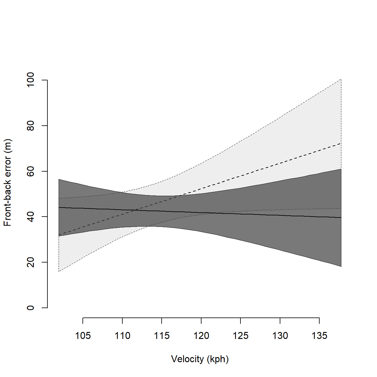
Based on the full sample of 30 fixed-wing locations, the estimated intercept and slope coefficient for airspeed in the front-back direction were 45.48 (C.I. = 36.48–54.26) and 8.95 (C.I. = -0.1–17.92) showing strong evidence for positive measurement bias in the direction of travel that increased approximately 9 m with each increase of 1 kph in airspeed (Table 1). The estimate for the same slope coefficient based on data excluding the most influential outlier was -0.99 (C.I. = -7.86–5.88) indicating airspeed had little to no effect. Removing the outlier resulted in a similar estimate (42.61, C.I. = 35.82–49.29) for the intercept in the front-back direction again suggesting location measurements were biased >40 m in the direction of travel. Intercept and slope estimates in the left-right direction for the full and reduced data sets were similar, and did not show evidence of substantial bias in or influence of airspeed on error perpendicular to direction of travel in fixed-wing aircraft. Parameter estimates for each direction based on the intercept-only model also were similar between data sets with all indicating strong evidence for positive bias in the front-back direction and lack of strong evidence for any bias in the left-right direction (Fig. 2). For the helicopter-based locations, both the full and reduced data set with outlier removed showed strong support for GPS locations being substantially biased westwardly by approximately 30 m and northly by approximately 20 m.

Precision of location measurements, estimated in our models as standard deviation was similar (range = 15.8–16.4) across models and data sets for fixed-wing measurement errors in the left-right direction. Conversely, removing the outlier location from fixed-wing analysis improved precision (i.e., lowered in the front-back direction for both models, with declining approximately 8 and 6 m for intercept-only and intercept-slope models, respectively. For the helicopter-based trials, removing the outlier improved precision in both cardinal directions, although precision improved more in the east-west direction (decline of 6 m) than the north-south direction (decline of 2 m).
Misclassification analysis
Estimates of misclassification probabilities for fixed-wing trials, assuming locations are georeferenced to 30-m resolution spatial data, indicated that the probability of an animal location obtained using our data collection methods being misclassified in the left-right direction was 0.37 (C.I. = 0.24–0.50), and the probability in the front-back direction was 0.94 (C.I. = 0.85–0.98). When assuming coarser spatial resolutions of 90-m and 250-m, only misclassification probability in the front-back direction at the 90-m scale was substantially greater than 0 (θ = 0.45, C.I. = 0.31–0.59, Table 2). For helicopter trials, estimated probabilities were 0.93 (C.I. = 0.84–0.98) in the east-west direction and 0.67 (C.I. = 0.55–0.78) in the north-south direction when georeferenced to 30-m resolution spatial data. At 90-m resolution, misclassification probabilities would be relatively lower but still non-negligible at 0.14 (C.I. = 0.05–0.25) and 0.10 (C.I. = 0.04–0.21) in the east-west and north-south directions. As with the fixed-wing trials, misclassification probabilities essentially were zero in both directions at a 250-m resolution.
DISCUSSION
Results from our analyses confirmed our expectation that animal locations collected from fixed-wing aircraft using the equipment and protocols implemented in our simulated survey generally were biased in the direction of travel and unbiased perpendicular to the direction of travel. The average magnitude of bias we observed in the direction of travel (approximately 45 m) was unexpected due to the strict adherence to protocols by the pilot and observer to consistently time the collection of GPS locations when directly over the target. Given this consistency, we suspect a time lag from when the observer hit the mark button on the handheld GPS device to when the device recorded a location was a likely source of our observed measurement bias. Other sources of potential bias worth noting include observer fatigue, sun glare, and sighting angles. Our fixed-wing results also provided evidence to conclude that variation in airspeed during our surveys did not significantly contribute additional bias to animal locations. This evidence was not surprising because the protocol for our fixed-wing survey required the pilot maintain a consistent airspeed when each location was collected, which was reflected in observed airspeeds approximated from GPS track points that had a relatively low standard deviation of 8 kph compared to a mean airspeed of 114 kph. Although we had no a priori expectations for location precision, estimates of were higher (≥16 m) and precision was lower than may be desired for evaluating wildlife-habitat relationships at relatively small spatial scales.
Locations collected during our simulated helicopter survey were biased to the north and west regardless of whether the outlier location was removed. Such systematic bias was surprising given our data collection protocol for this survey instructed the pilot to hover directly over the target until the observer recorded a location in the GPS. We hypothesize the observed bias was caused by high winds observed during our simulated helicopter survey conducted 1200–1300 on 29 April 2022. Winds reported (Weather Underground 1995) during the noon hour at nearby Bethel, Alaska primarily came from the east at average speeds of 27 kph and gusts up to 40 kph. We believe strong easterly winds combined with the added effect of an open lake to the east of our target location likely caused the helicopter to rapidly drift to the west and north as the pilot released from hovering over the target immediately after a location measurement was collected. As in our fixed-wing survey, we suspect this abrupt movement combined with a time lag between the observer pressing a button to mark a location on the GPS device and when the device truly records the location may have caused the bias observed in our helicopter-based location measurements. Also as in our fixed-wing survey, we had no a priori expectations for location precision, however, estimates of again were higher (range = 12–21 m) and precision was lower than may be desired for evaluating wildlife-habitat relationships at fine spatial resolutions.
For both survey platforms, we discovered substantial bias and low precision in location measurements that have implications for designing aerial surveys to evaluate wildlife-habitat relationships. Ecological processes driving wildlife-habitat relationships, such as animal resource selection and species distribution, have long been known to vary across spatial scales (D. H. Johnson, 1980; Wiens, 1989). Therefore, research and monitoring projects designed to evaluate wildlife-habitat relationships must carefully match their sampling designs and data collection protocols with the spatial scale of ecological processes being investigated. In this case study, the data collection protocols used to collect animal locations during aerial surveys were not adequate to reliably georeference those locations to rasterized data at the relatively fine spatial scales (e.g., 30-m and 90-m) common in analyses of animal resource selection and species distribution. For example, our results demonstrated that even when measurement bias was negligible (i.e., left-right direction for the fixed-wing survey), considerable imprecision of our location measurements resulted in a 37% misclassification rate that would likely lead to estimation problems in subsequent analyses. Conversely, our methods did appear to be adequate to collect animal location data with sufficient accuracy and precision for analyses at larger spatial resolutions such as 250-m.
For research and monitoring of wildlife populations over large, inaccessible landscapes, aerial surveys will continue to be a primary method of data collection for the foreseeable future. When objectives for such surveys include evaluating wildlife-habitat relationships by relating animal locations to spatial environmental data, we offer several recommendations to overcome or circumvent problems caused by measurement error. Our first is to clearly identify the spatial scale(s) of wildlife-habitat relationships of interest and the scale, accuracy, and precision of animal locations and spatial data required for analysis. We next recommend careful design and thorough testing of data collection methods to evaluate location accuracy and precision like those used in this case study, and we emphasize the importance of field staff training to maximize accuracy and precision. During our study, we found considerable value in the pilot and observer co-developing and practicing protocols for aircraft maneuvering and data collection prior to conducting the survey, which we believe allowed us to rule out some potential sources of bias. However, we also recognize the simple experimental design of this study restricted data collection to a single location on a single day by a single pilot-observer pair marking a fixed, non-moving location during identical weather conditions thus limiting inferential strength and generalizability of our results to evaluate potential biases of aerial surveys conducted under different circumstances.
As demonstrated by this study, operationally testing field data collection methods by quantifying the types and magnitude of measurement error can be important for discovering previously unknown sources of measurement bias. Based on the frequency and influence of measurement outliers in our evaluation, we also call attention to the importance of proper sampling design and sample size to ensure a robust evaluation. If all feasible options for minimizing measurement bias and maximizing precision have been implemented during data collection and measurement error still exceeds survey objectives, we recommend using one of many analytical methods designed to correct or compensate for measurement errors in animal location data. As a starting point, we recommend becoming familiar with the body of literature on location errors for GPS-equipped animal tracking devices (Frair et al., 2004, 2010).
Acknowledgments
We acknowledge the U.S. Fish and Wildlife Service for supporting this study. We thank S. Hermens and the late R. Sundown for their roles as pilots for this study.